Simulated datasets for statistical analysis — simulated

A collection of six simulated datasets representing different combinations of distributional assumptions, variance homogeneity, and sample-size balance. These datasets are designed for demonstrating and evaluating statistical procedures under a range of common experimental conditions.

Usage

O_O_O

O_O_X

O_X_X

X_O_O

X_X_O

X_X_X

Format

Six data frames, each containing the following two variables:

grp: Character vector identifying the experimental group.
val: Numeric vector containing the simulated response values.

The number of observations differs according to the experimental design: balanced datasets contain 120 observations (20 per group), whereas unbalanced datasets contain 128 observations with group sizes of 27, 24, 16, 30, 11, and 20.

An object of class data.frame with 120 rows and 2 columns.

An object of class data.frame with 128 rows and 2 columns.

An object of class data.frame with 120 rows and 2 columns.

An object of class data.frame with 110 rows and 2 columns.

Details

All datasets contain six groups (G1 to G6) and two variables:

grp: A character variable identifying the group.
val: A numeric response variable.

The dataset names follow a three-character notation separated by underscores: D_V_B, where each position describes a different property of the data:

First position (D): Distribution. O indicates normally distributed data, whereas X indicates distribution-free or non-normally distributed data.
Second position (V): Variance. O indicates homoscedasticity, whereas X indicates heteroscedasticity.
Third position (B): Design balance. O indicates a balanced design, whereas X indicates an unbalanced design.

The six datasets are:

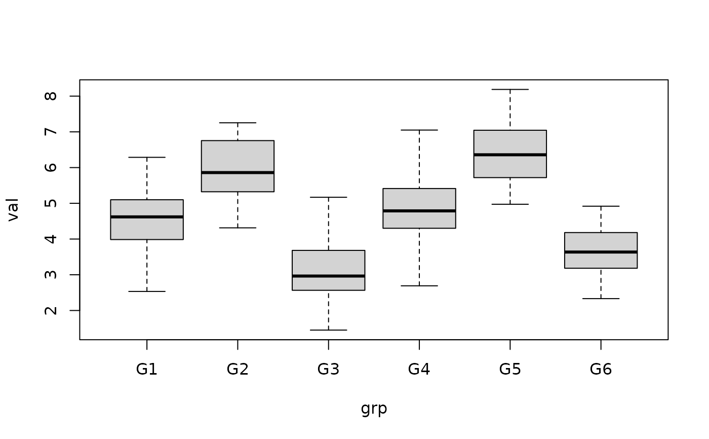
O_O_O: Normally distributed, homoscedastic, and balanced-designed data. Each group contains 20 observations.
O_O_X: Normally distributed, homoscedastic, and unbalanced-designed data. The group sample sizes are 27, 24, 16, 30, 11, and 20, respectively.
O_X_X: Normally distributed, heteroscedastic, and unbalanced-designed data. The group sample sizes are 27, 24, 16, 30, 11, and 20, respectively.
X_O_O: Distribution-free or non-normally distributed, homoscedastic, and balanced-designed data. Each group contains 20 observations.
X_X_O: Distribution-free or non-normally distributed, heteroscedastic, and balanced-designed data. Each group contains 20 observations.
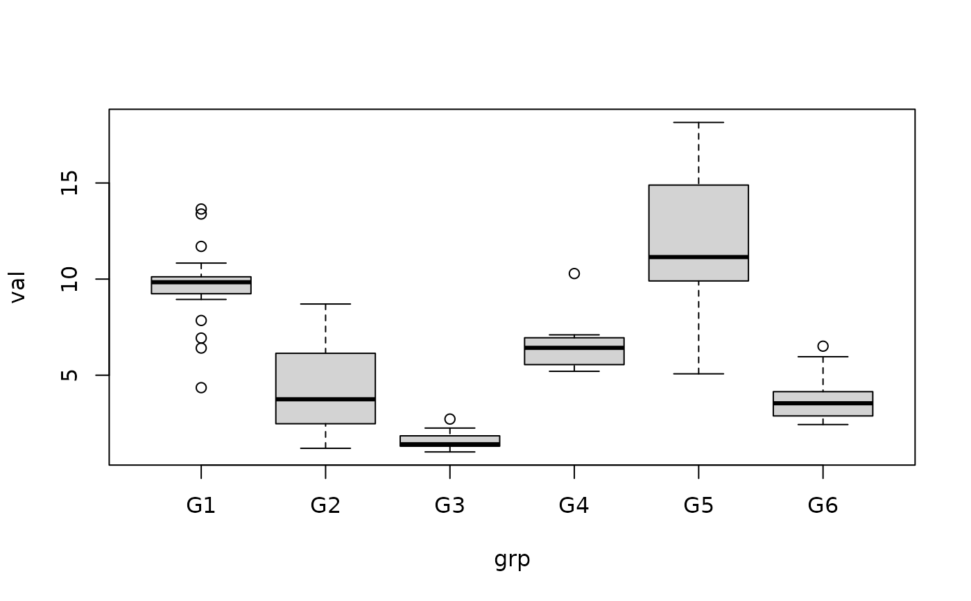
X_X_X: Distribution-free or non-normally distributed, heteroscedastic, and unbalanced-designed data. The group sample sizes are 27, 24, 16, 30, 11, and 20, respectively.

The normally distributed datasets were generated using stats::rnorm(). The distribution-free datasets were generated using combinations of stats::rcauchy(), stats::runif(), and stats::rgamma(), together with stats::rnorm(). Different location and scale parameters were used to produce the intended distributional and variance characteristics.

These datasets are intended for methodological examples, unit tests, demonstrations, and comparisons of statistical procedures under different combinations of assumptions. They should not be interpreted as empirical observations from a real population.

Dataset characteristics

Dataset	Distribution	Variance	Design
`O_O_O`	Normal	Homoscedastic	Balanced
`O_O_X`	Normal	Homoscedastic	Unbalanced
`O_X_X`	Normal	Heteroscedastic	Unbalanced
`X_O_O`	Non-normal	Homoscedastic	Balanced
`X_X_O`	Non-normal	Heteroscedastic	Balanced
`X_X_X`	Non-normal	Heteroscedastic	Unbalanced

Examples

data(O_O_O)

boxplot(val ~ grp, data = O_O_O)


data(X_X_X)

boxplot(val ~ grp, data = X_X_X)


aggregate(val ~ grp, data = O_O_O, FUN = mean)
#>   grp      val
#> 1  G1 4.641624
#> 2  G2 5.948743
#> 3  G3 3.106485
#> 4  G4 4.880083
#> 5  G5 6.375095
#> 6  G6 3.640620

aggregate(val ~ grp, data = X_X_X, FUN = mean)
#>   grp       val
#> 1  G1  9.667313
#> 2  G2  4.302930
#> 3  G3  1.566811
#> 4  G4  6.490958
#> 5  G5 11.823754
#> 6  G6  3.790654